Mgr.inz.arch. Makowska Agnieszka
Cracow University of
Technology
COMPUTER AIDING FOR ESTIMATING THE
CURVILINEAR ENGIEERING STRUCTURES
1.Introduction
This paper is the continuation of determining
of the curvelinear objects parameters.
The
most of contemporary building use soft form and irregular shapes.
The
base of the cost calculation is the exact calculation of length or the surface
area or the volume. The new techniques and technology use very expensive
materials, hence it is very important to do the precise calculation to reduce
the cost of investment.
Exact
calculation of the surface or the volume of straight-line forms is easy, in the
case of curvilinear objects it can be controversial.
The
attempt of description of curvilinear objects made with the help of cubic
spline interpolation has been presented in this paper.
2. Elementary theory of
cubic spline
We have got n+1 points in the interval <a,b>
: a= x0 , x1 ,
. . . , xn = b, call this nodes and value function y=f(x) in
this points: f(x0)=y0 , f(x1), ...,f(xn).
Pair (xk, yk) we call data points.
We seek estimate values function f(x) class C2 between nodes as of polynomial of third
degree for x![]() <xi-1, xi>.
Let us mark us:
<xi-1, xi>.
Let us mark us:
![]()
![]() for i=0,1,2,...,n (1)
for i=0,1,2,...,n (1)
from definition of function f(x) to appear that f’’(x)
is the continuous function in interval
<a ,b> and linear for x![]() <xi-1, xi>, so we have:
<xi-1, xi>, so we have:
![]() (2)
(2)
where: ![]()
Integrating twice (2) we obtain:
![]()
(3)
where
(4)
Using
function’s conditions of continuity and first derivative by algebraic
conversion we have linear system of equation :
![]() for
i=1,…,n-1 (5)
for
i=1,…,n-1 (5)
where: ![]()
![]()
![]()
 for
i=1,2,..,n-1 (6)
for
i=1,2,..,n-1 (6)
System (5) has got n-1 equations and n+1 unknown
coefficients: M0, M1,..., Mn .
Often we accept two additional
conditions :
M0=0, Mn=0 (f”(x0)=0, f”(xn )=0:
Natural cubic Spline).
Let us mark as :
![]() for i=2,3,...,n-1 (7)
for i=2,3,...,n-1 (7)
![]() for
i=2,3,...,n-1 (8)
for
i=2,3,...,n-1 (8)
and for symmetric expression :
![]() .
. ![]() (9)
(9)
From the first equation of system (5)
![]() we have:
we have:
![]() , or
, or
![]()
by recurrence
end algebraic conversion we obtain:
![]() , for
k=1,...,n-2 (10)
, for
k=1,...,n-2 (10)
Using principle of mathematical induction easily proof
the truth of this expression.
From
the last equation of system (5) ,we have:
![]() (11)
(11)
after
calculation coefficients Mk
we construct function f(x):
(12)
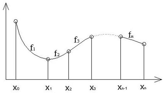
Fig.1 The visual graph of function
f[x]
where fi is the
right side of expression (3).
We define Heaviside’s function:
![]()
and then function f(x) is expressed one rule:
![]() (13)
(13)
Now we can write in any
programming language the basic procedure named splajnP, in which the input
parameters are data points: (x0,y0) , (x1,y1)
, . . . , (xn,yn)
, and on the exit of that procedure we will get function f(x) and her graph.
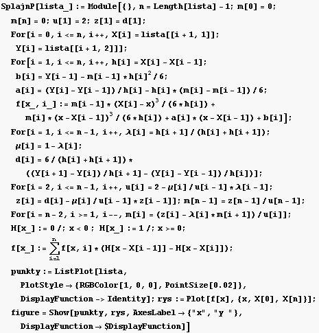
Fig.2 Procedure SplajnP written in Mathematica program
3. Application and estimation of error
Example
1.
In
publications or WEB we can often see graph of function, but we do not know
value of this function. We will show in three steps, how can we find a rule of
function.
1.
step: we import a scanned graph of function to the Mathematica program
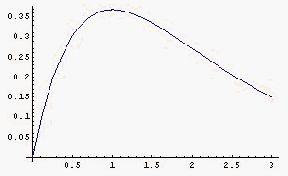
Fig.3 Graph of unknown function g[x]
2 step: we read and write coordinates of screen witch
Fig.3:
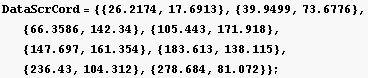
Fig.4 Coordinates of screen function g[x]
We read coordinates of beginning (xB, yB) and end (xE,yE) of graph and corresponding them
coordinates of screen are: (xBS,yBS) and
(xES,yES).
Now we define a procedure using linear interpolation
which will transform coordinates of screen on coordinates of real:
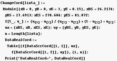
Fig.5 ChangeCord procedure
After executing of this procedure with parameters
DataScrCord we obtain real coordinates:
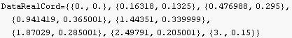
Fig.6 Real coordinates
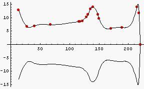
Step 3: we evaluated procedure SplajnP [DataRealCord]
and we obtain function f[x] and her graph :
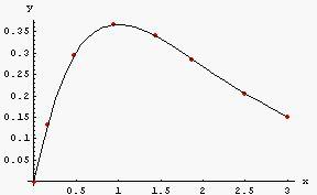
Fig.7. f[x] Function graph
The compatibility of Fig.3 and Fig.7 is almost ideal,
author knows g function:
g[x]=x Exp[-x] , therefore we can find estimate error
in this method:
![]()
![]()
Fig 8. Estimate error
Adding
graphic and numeric instructions to procedure SplajnP we can obtain new
procedures.
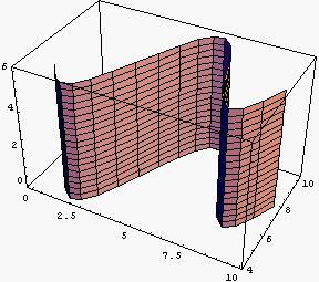
Example 2. In the procedure SplajnTheWall the first parameter are
data points, and the second is height of the wall; output parameters are the
graph and area of the wall surface.
![]()
Fig.9 Result of Procedure
SplajnTheWall[data,4]
Example 3. We construct the circle with centre on curve and in normal
plane which moves after curve.
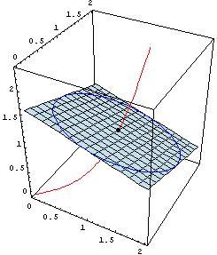
Fig.10 The circle in normal plane
In the SplajnPipeline procedure the first parameter are data points, and
the second is radius of pipeline; parameters output are graph and area of the
pipeline surface.
![]()
![]()
Fig.11 Result of Procedure
SplajnPipeline [data,0.7]
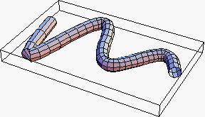
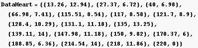
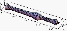
Example 4. In the SplajnVolume procedure input parameter are data
points, output parameters are graph and volume of the solid formed by the
revolution of the curve y=f[x] around x-axis.
![]()
Fig.12 Result of Procedure
SplajnVolume[DataHeart]
Fig.12 represents the heart of Zygmunt’s bell.
These
calculations were made without taking into account of the handle of the bell
heart. The mass of the handle was estimated as 20 kg. The density of the heart is unknown, there
are some admixtures: phosphorus, sulphur, etc. According to the accessible data
new heart mass is about 350 kg. Specific mass of the heart is assumpted as 7.7
[g/cm3].
Counted
mass of bell: mass=47371.7[cm3]*7.7[g/cm3]/1000+20[kg]=384.762
[kg], error of calculations=(384.762 –350)/350*100% = 9.9 %
The heart of Zygmunt Bell is in the Wawel
Cathedral in Cracow.
Conclusion
The presented above method of calculations enables the
precise defining of the necessary object parameters to its optimalization from
the engineer’s point of view, for example the quantity of necessary material to
object construction. The presented method of calculations permits to
qualify of object with engineering point of view permits his optimization
necessary parameters. The method creates the possibility of the objects
modelling as well as quick amendments of parameters in the project process. On
the base of support of prepared procedures in Mathematica program, it permits
to calculate the interesting us parameters.
Literature
[1].Stephen
Wolfram Mathematica 4 book: Cambridge Universuty Press 1999.
[2]. Z. Fortuna D.Macukow.
J.Wasowski: Metody numeryczne WNT Warszawa 1982.
Abstract
The natural cubic splain theory elements apllied to building engineering have been presented in the paper. Coefficients of cubic spline have been determined in recurring form. Graphics and numerical procedures were executed in programme "Mathematica". Application of that theory for estimating of curvilinear objects has been presented on chosen examples.